Issue, No.12 (December 2019)

Can We Obtain Better Distributional Measures Correcting for Differential Unit Non-Response Bias in Household Surveys? An Illustration Using Data from the US Current Population Survey

by Salvatore Morelli, (Stone Center on Socio-Economic Inequality, Graduate Center, City University of New York (CUNY)), and Ercio Munoz, (Graduate Center, City University of New York (CUNY))

Recent literature on economic inequality has focused a great deal of attention on the estimation of income concentration measures (e.g., the share of total income held by a small, rich segment of the population). One of the key findings of this new stream of literature is that estimates of income concentrations as derived from tax-administrative sources are generally higher and show a stronger positive trend than what is estimated via household survey data, especially for very high-end income groups.

Differences can be quite large at the very top, but relatively small as we move further down the income pyramid. Figure 1 depicts the existing gap between top income shares in the US as estimated from IRS tax data versus data from the household survey from the Current Population Survey (CPS).

Certainly, part of the difference can be reconciled by using similar units of analysis and income concepts between data sources, as shown in the figure below. Yet this strategy is not sufficient to fully explain the discrepancy in income shares obtained through the different sources.

Figure 1: Reconciling measures of top income shares across tax and survey data

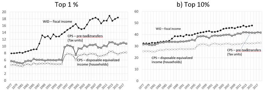
Notes: data elaboration by the authors on CPS data. WID series is taken from wid.world

There is a growing recognition that household survey data may be less suitable than administrative sources to capture all income sources at the very top for a variety of reasons linked to the quality of the measurement of the upper tail of the distribution. There are, broadly speaking, two main problems. First, without an appropriate oversampling strategy for rich households, surveys might run into problems with small samples, which increase statistical volatility and can distort our representation of highly skewed distributions, such as those for income or wealth. Second, in survey data, non-random households may not be reachable, or willing to cooperate, or to disclose full information about their economic and financial conditions.

This note focuses specifically on the effect of differential unit non-response on key distributional measures; we do not address fundamental question of efficient sample design. Sample designs can have substantial, perhaps even larger, implications for estimates of concentration and inequality.

The growth of unit non-response in household surveys

Unit non-response rates in household surveys (i.e., the share of non-respondent households among total households that are sampled) have been increasing in recent decades (Meyer et al. 2015) and household surveys in the US are no exception. In the CPS, the aggregate non-response rate more than tripled between 1977 and 2018, increasing from approximately 4% to more than 14%.

Figure 2. The rate of unit non-response in the US CPS data (1977-2018)

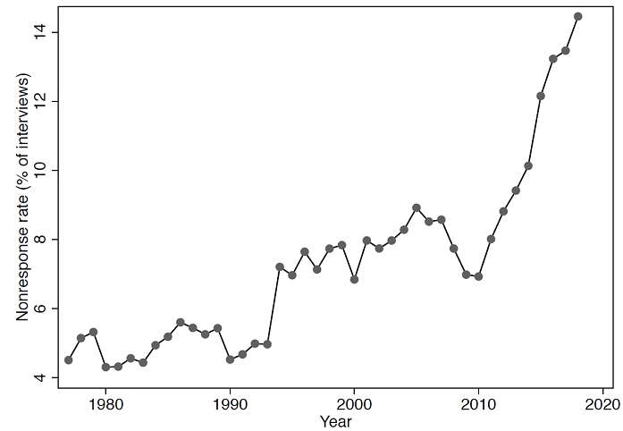
Notes: Data elaboration by the authors on CPS data

As reported in Atkinson and Micklewright (1983), rising aggregate unit non-response rates may not necessarily create biases in estimations of the moments of income distribution, as long as the non-response pattern is random. However, there is growing evidence that unit non-response (e.g., missing households) and item non-response (e.g., missing specific information about the households) are directly associated with the economic status of the sampled households, such as their total income or wealth, among other characteristics.

This evidence is problematic. Kennickell (2019), in his introduction, argues that “[i]f differences in willingness of sample members to participate are not statistically independent with respect to the analytical dimension(s) of interest, then the measured distribution will differ from what would be estimated from the full sample and many classes of estimates made on such data will be biased”. At the same time, Kennickell (2019) acknowledges, in his conclusions, that “[t]his fact appears to be insufficiently recognized by many practitioners who find ‘significant’ relationships when comparing estimates from different surveys”. However, he suggests that “[s]ometimes data are available for calibration to address non-random effects in the response mechanism”.

How then can we utilize information on differential unit non-response to adjust household income survey data to obtain better distributional estimates?

Accounting for differential unit non-response

It is, in principle, possible to address the issue of differential unit non-response along the income distribution without resorting to external administrative sources of data – which are typically difficult to access – other than the household survey.

Korinek et al. (2006, 2007) show how the latent income effect on household compliance (i.e. probability of response) can be consistently estimated with the available data on average response rates by any sampling strata. The information about the probability of non-response, estimated at the household level, could then be used to correct survey weights (e.g. to give more weight to those households that have lower probabilities of responding because of their high income level).

In practice, publicly available information on response rates is often available by geographic areas only (e.g., regions or sub regions). Indeed, Korinek et al. (2007) proposed a novel estimator to compute a survey compliance function using regional non-response rates. The estimator is based on the following moment condition for region j (with j ∈ J ), where J is the total number of regions:

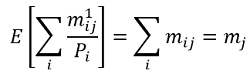
where m¹_ij is the total number of households with income i in region j that comply with the survey, m_ij is the total (unobserved) number of households with income i in region j, m_j is the total number of households sampled in region j, and P_i is the probability of response for household with income i.

Using CPS data from 1998 to 2004, Korinek et al. (2007) find a highly significant negative effect of income on survey unit response, which may bias income inequality estimates.

Munoz and Morelli (2019) present a new Stata command to implement this method, <kmr>. To illustrate its use, the authors use data from the 2018 CPS downloaded from IPUMS (Flood et al. 2018), merged with the number of interviews and Type A non-responses (interviewer finds the household’s address but obtains no interviews) obtained from the NBER CPS Supplements website. These data are sufficient to derive state-level non-response rates in the US, defined as Type A non-responses as a share of the sum of interviewed households and Type A non-responses. Figure 3 below reports geographical variation in non-response rates across the US states.

Figure 3 CPS unit non-response rates by US States. 2018

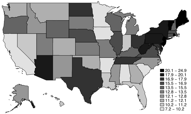
Notes: Data elaboration by the authors on CPS data.

These data (described above) are used to estimate the probability of response as a function of total household gross income per capita. Gross income is factor income plus all public and private monetary transfers received, minus taxes paid. The estimates are in turn used to generate a set of corrected weights which allow re-estimation of distributional variables (e.g., Gini coefficients).

To illustrate the implications of Korinek et al.’s suggested correction method, Morelli and Munoz (2019) estimate the compliance function in the CPS data using the full set of available years, from 1977 to 2018, and show the effect that such weights-corrections may have on income inequality, income concentration, and income poverty. The compliance functions can be estimated for both pooled years or individual years. We illustrate the latter approach here.

Figure 4 indicates that all compliance functions, estimated for all available CPS waves, tell a similar story, namely that high levels of total household income are associated with systematically lower levels of response probability. The estimated compliance functions can then be used to adjust the survey weights. In other words, the few observations of rich households available in the sample of respondents will be given more weight. Figure 4 also suggests that lower compliance rates can also be found at the bottom of the distribution, suggesting that both tails of the income distribution should be given bigger weight.

Ideally, this type of adjustment ought to be applied using raw survey weights, before any corrections to the weights are implemented by the institutions administering the survey. However, raw survey weights are not generally available outside the data-producing institution. Hence, for the purpose of this exercise, we adjust weights that are assumed to be equal to 1.

Figure 4 Estimated probability of response by total household income per capita using CPS data (1977-2018)

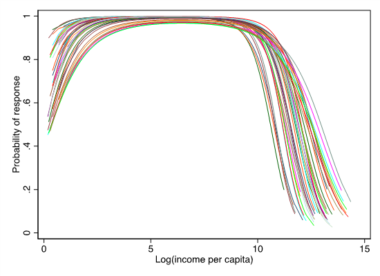
Notes: Data elaboration by the authors on CPS data.

Figure 5 Correction of survey weights controlling for differential unit non-response bias: average % effect on distributional and poverty measures using CPS data (1977-2018)

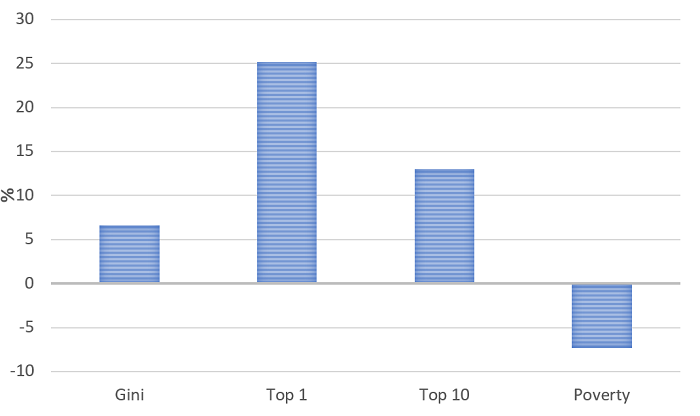
Notes: Data elaboration by the authors on CPS data.

Concluding remarks

Unit non-response rates, in the CPS data, grew significantly between 1977 and 2018. Given the direct connection between non-response probability and household income levels, the use of uncorrected income survey data may result in biased estimates of income distribution measures. In this note, we have illustrated how one correction method proposed by Korinek et al. (2007) works and how it can be implemented easily with a new user-written command in Stata, <kmr>.

By applying the method by Korinek et al. (2007) on CPS data for each year from 1977 to 2018 we estimate an average positive correction of 6.6% for the Gini coefficient and average negative correction of 7.3% for the poverty rates. The top 1%, instead, may be underestimated by approximately 25% (see Figure 5).

Given the profound policy implications of such an exercise, we emphasize that more research is needed, for a variety of reasons.

First, there is large year by year variability underlying the estimated average correction rates. Moreover, the average adjustments are sensitive to whether the compliance function is estimated by pooling years of observations or not.

Second, and as pointed out in Deaton (2005), the correction for unit non-response may also result in inequality estimates that could be lower than the uncorrected ones: “…with greater non-response by the rich, there can be no general supposition that estimated inequality will be biased either up or down by the selective undersampling of richer households. (The intuition that selective removal of the rich should reduce measured inequality, which is sometimes stated as obvious in the literature, is false, perhaps because it takes no account of reduction in the mean from the selection.)” (p. 11).

Third, the correction results may be sensitive to the number of regions considered (Hlasny and Verme, 2018).

Fourth, the method described here relies solely on within-survey data and pure re-weighting with no replacing of observations and provides reasonable results under the condition that the maximum income reported in the household survey data is not too dissimilar from the “real” maximum income (i.e., the support of the income distribution is the same). This condition is usually not met. To overcome this main limitation, new fruitful avenues of research include merging household survey data with external information (e.g. tax administrative sources), before modifying survey weights (Blanchet, Flores, and Morgan, 2019).

Although, different correction methods might agree on the fact that income distribution estimates are misrepresented using household survey data, analysts would ideally combine multiple correction approaches to reach reasonable conclusions about the extent and direction of such biases.

References

Atkinson, A., & J. Micklewright (1983). ‘On the Reliability of Income Data in the Family Expenditure Survey 1970- 1977’. Journal of the Royal Statistical Society, 146(1), 33-61. doi:10.2307/2981487

Blanchet, T., I. Flores, and M. Morgan (2019). The Weight of the Rich: Improving Surveys Using Tax Data. Unpublished manuscript.

Bollinger, C, B. Hirsch, C. Hokayem, and J. Ziliak (2019). ‘Trouble in the Tails? What We Know about Earnings Nonresponse 30 Years after Lillard, Smith, and Welch’. Journal of Political Economy, 127, no. 5 (October 2019): 2143-2185.

Deaton, A. (2005). ‘Measuring Poverty in a Growing World (or Measuring Growth in a Poor World)’, The Review of Economics and Statistics, 87:1, 1-19

Flood, S., M. King, R. Rodgers, S. Ruggles, and R. Warren (2018). Integrated Public Use Microdata Series, Current Population Survey: Version 6.0 [dataset]. Minneapolis, MN: IPUMS. doi: https://doi.org/10.18128/D030.V6.0.

Hlasny, V. and P. Verme (2018). ‘Top Incomes and the Measurement of Inequality in Egypt’, The World Bank Economic Review, vol. 32, Issue 2, 428–455.

Kennickell, A. (2019). ‘The tail that wags: differences in effective right tail coverage and estimates of wealth inequality’. The Journal of Economic Inequality , vol. 17(4), 443-459, December.

Lustig, N. (2019). The “Missing rich” in Household Surveys: Causes and Correction Approaches. CEQ Working Paper 75.

Meyer, B. & W. Mok & J. Sullivan (2015). ‘Household Surveys in Crisis. Journal of Economic Perspectives’, American Economic Association, vol. 29(4), 199-226.

Morelli, S. and E. Munoz (2019). Unit Nonresponse Bias in the Current Population Survey. Unpublished manuscript.

Munoz, E. and S. Morelli (2019). kmr: A Command to Correct Survey Weights for Unit Nonresponse using Group’s Response Rates. Unpublished manuscript.