Issue, No.14 (June 2020)
R-Charts in LISSY X: A Short Guide
In the beginning of June 2020 LIS has launched a quite innovative version of LISSY, a fully web-based interface that includes graphing functionality. For all non-users of LIS databases, since LIS’ early days, LISSY is the heart of data services at LIS. LISSY is the remote execution system that allows researchers to access LIS and LWS microdata remotely. Users of this interface can write and submit statistical requests in R, SAS, SPSS and Stata. This latest update includes the option to display charts on screen and export them as image, to review earlier jobs in a multiple jobs window, to download of all results in PDF/TXT/PNG format, and to import of syntax files into the job editor panel.
Thus in order to get you started working with the new LISSY, we have produced an example of R code that allows users to easily import and clean LIS and LWS data as well as to produce some basic indicators. The whole code can be found and downloaded online. In this short exercise, we will:
- Show how to perform data transformations in R;
- Use these data and estimate Gini coefficients;
- Plot and export examples of the Lorenz Curve.
Curious? Ok so let us look at each point in more detail.
The first thing that we need to do is to start the R session by loading the required packages and functions. For this exercise we load the following R packages:
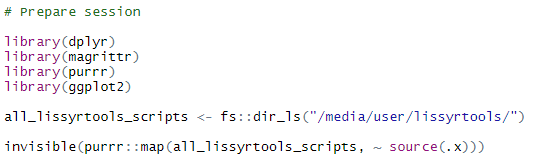
The code above loads four packages and then reads all the functions stored within the ‘lissyrtools’ directory. Additional documentation on these functions, such as arguments and examples of use can be found here.
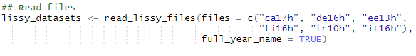
The ‘read_lissy_files()’ function will let you import one or multiple files, specified as a character vector in the first argument (named ‘files’). Under the hood, the function returns a list with the imported files as elements. In this example, the list is stored as ‘lissy_datasets’ and would contain six elements, one for each imported dataset. The second argument of the function (‘full_year_name’) will allow you to obtain the names of the files with four digit years (e.g. ‘ca2017h’ instead of ‘ca17h’). This can be convenient when performing certain actions, as four digit years can be more easily sorted.
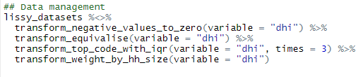
Now that we have imported the datasets we will prepare them for analysis. For this, ‘lissyrtools’ offers a set of ‘transform_’ functions such as the ones in the following chunk of code:
In case you are not familiar with the R package ‘magrittr’, ‘%>%’ and ‘%<>%’ are pipes that allow to pass the result of one function as the first argument of the next one. Additionally, ‘%<>%’ stores the result back to the left-hand-side object passed. Functions in ‘lissyrtools’ are compatible with these pipes as they make the code much easier to read. The ‘tidyverse’ website has great articles on the use of pipes in R code.
The ‘transform_’ functions above, process the files previously stored as ‘lissy_datasets’ with the following:
- ‘transform_negative_values_to_zero(variable = “dhi”)’ recodes all negative values to zero in the selected variable ‘dhi’- – Disposable household income.
- `transform_equivalise(variable = “dhi”)’ adjusts the selected variable by square root of the number of household members.
- ‘transform_top_code_with_iqr(variable = “dhi”, times = 3)’ applies an upper limit to the variable. This corresponds to 3 times the Interquartile Range of the variable transformed using the natural logarithm.
- ‘transform_weight_by_hh_size(variable = “dhi”)’ multiplies the weight by the number of people in the household.
Notice that, as we used the ‘%<>%’ pipe, all transformations are automatically stored back to ‘lissy_datasets’.
The computation of estimates can be done with the ‘print_indicator()’ function as shown below. Before that, we might want to perform a last transformation – ‘transform_adjust_by_lisppp’- which adjusts by a combination of CPI and PPP (see our page on PPP Deflators) to make data in different currencies, countries and years comparable. The ‘print_indicator()’ function can currently compute the mean, median, percentile ratio, and Gini coefficient. If there are missing values in the variable, ‘na.rm = TRUE’ should be specified. Otherwise the function will return NAs as estimates. This is done so users don’t compute estimates and accidentally ignore missing values.

The previous code prints out the estimated Gini coefficients for the files in ‘lissy_datasets’.

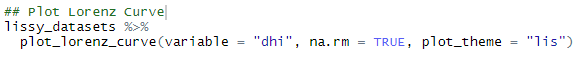
Now, we will explore the possibilities that the new version of LISSY offers by producing some graphs. The following two chunks of code produce two different plots. Thus, they should be written on separate LISSY jobs. Otherwise, LISSY overwrites the later graph with the first one.
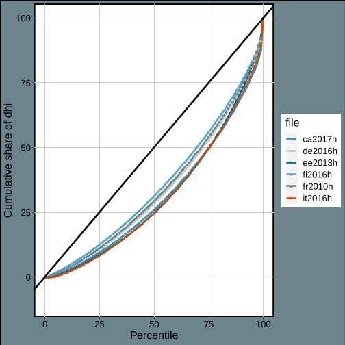
We can plot the Lorenz curve for a variable of all imported datasets with the ‘plot_lorenz_curve()’ function. Again, you must make sure that missing values are explicitly removed. The function also has an optional ‘plot_theme’ argument, which currently supports only a limited number of options.
.
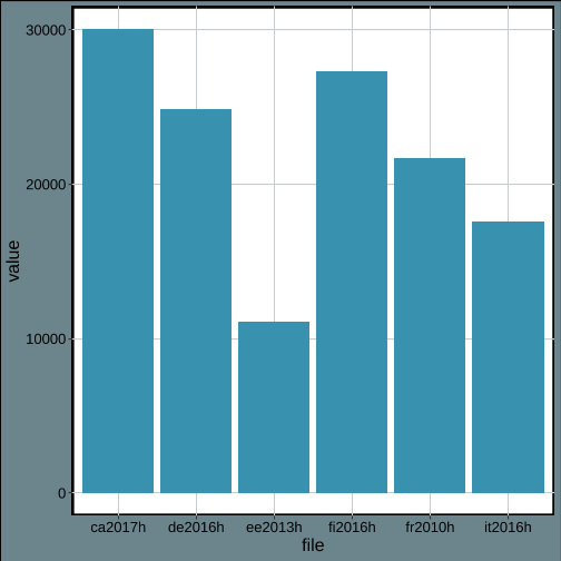
Similar to‘print_indicator()’, the ‘plot_indicator()’ function computes and displays the plot for a function. In the code below we apply again the deflation adjustment and then choose the median as indicator. The graph obtained from LISSY is shown below the code.

We hope that we could show you with this short data exercise, how easy cross-national data can be explored. For questions or suggestions about the code above, please email our data support team at usersupport@lisdatacenter.org . We are eager to receive your feedback.