Issue, No.15 (September 2020)

Top and Bottom Coding at LIS

by Jörg Neugschwender¹ (LIS)

Introduction

Since its foundation in the 1980s, LIS has acknowledged that even after harmonisation comparability concerns between household surveys from different countries could remain. Such differences arise mainly from national methodological procedures, when implementing representative surveys. In the beginning, this concerned mostly varying sample sizes and income units (Smeeding et al., 1985; O’Higgins et al., 1985, Atkinson et al., 1994). Later, differences in top coding practices by data providers and representativeness of the upper end of the income distribution (Gottschalk and Smeeding, 2000; Cowell and Flachaire, 2007) were discussed.

In order to keep true country rankings unbiased by nationally applied top coding procedures, the use of bottom and top coding techniques was proposed and disseminated. Besides others, Gottschalk and Smeeding (1997) and Smeeding (1997) implemented a top code of 10 times the median of disposable income, which equally served as a benchmark applied to the LIS Key Figures. Similarly, Fritzell (1992) applied a top coding value of 15 times the median in order to reduce the influence of extreme values at the top. At that time, Gottschalk and Smeeding (2000) reassured that LIS top coding had no influence on rank order and in general had a very limited influence on the Gini Index of advanced countries. Whereas this statement seemed a proper one for the advanced countries, Székely and Hilgert’s (1999) cross-national study of 18 national surveys from the LAC countries showcases well how underestimation of top incomes varies across countries in the region. Moreover, top coding practices are hardly found in LAC countries.

As the LIS Database has gradually grown to include more and more emerging economies, additional sensitivity analyses have become necessary. A main motivation of this paper is to reassess the influence of the previously applied top and bottom coding practices on the emerging economies. We acknowledge that the general idea of top and bottom coding is not unproblematic, as cutting the data at the extreme of maximum values could reduce inequality (when there is no measurement error in the data). On the other hand, when there is measurement error, it could turn out to be a plausible strategy to reduce variability in the tail distributions and to enforce a common practice to preserve ‘smoothened’ trends and country rankings between data sets with varying degrees of measurement error. We therefore aim to clarify whether the necessity to use top and bottom coding practices with the data at hand remains.

The following empirical section will show a sensitivity analysis for top coded and bottom coded incomes separately. Using the Gini Index we compare the previous top coding procedure (10 times the median of equivalised disposable income) with alternative measures, such as 20 times the median of equivalised disposable income and the detection of extreme values via the interquartile range (IQR). Likewise, we perform a sensitivity analysis for bottom coding techniques. The previous method (bottom coding at 1 % of the mean of equivalised disposable household income) is compared against bottom coding at value 0 and detection of extreme values via the interquartile range (IQR). In the final section, we will discuss why we adopted the practice of top and bottom coding at the lower and upper boundary for extreme values for the LIS Key-Figures and other indicators in LIS’ Data Access Research Tool (DART). Last, we briefly present more advanced statistical measures which are specifically intended for modelling the tails of the distribution.

Sensitivity Analysis of Bottom and Top Coding

First, we investigated the impact of different top coding procedures on the Gini Index for disposable household income (and likewise for wages). We computed three alternative measures in comparison to non-top-coded income.² The first one is the threshold that for many years has been put in place by LIS and which has been adopted by many LIS users, the top code at 10 times the median of disposable income. A second one simply raises the threshold to 20 times the median, to accommodate more unequal income distributions in the recently added emerging countries. And a third one, the interquartile range (IQR), is a common procedure that is applied to detect extreme values in distributions. The IQR is, for example, applied by the European Commission – Eurostat (2018) for the detection of outliers in the wage distribution; by reporting back to national agencies, data providers are asked to possibly confirm or correct for these values. A log transformation before defining the interquartile range takes into account that income is skewed to the right. Thus the upper boundary is defined as Q3*(Q3/Q1)^3.³ which is then used as a top code (see Figure 1). We therefore basically tested the impact of this technique as a strict top code.

Figure 1: Interquartile Range at the upper boundary

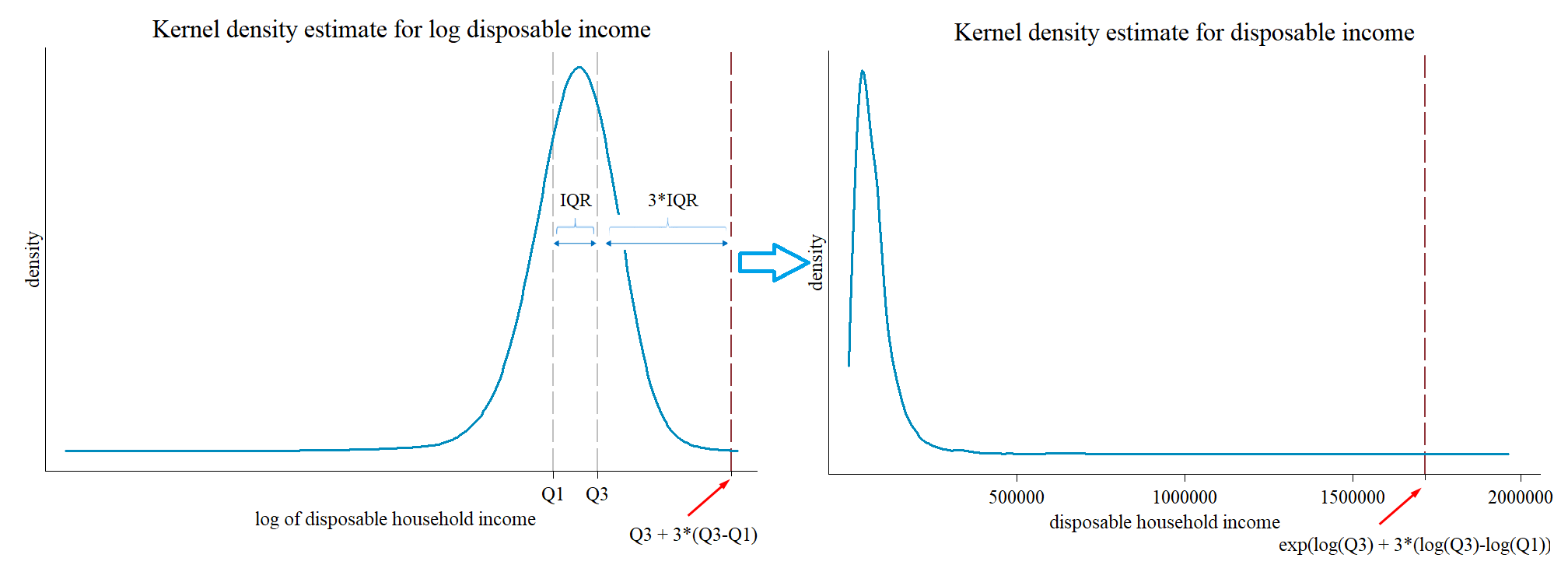
Figure 2 shows findings for the Gini Index on disposable household income (equivalised by the square root of household members) for selected countries. Equally, Figure 3 shows findings for wages. Many countries show that the IQR is much closer to the reference scenario of non-top-coded values. Particularly striking are the considerably lower Gini values in emerging economies when applying the 10 times the median threshold. Even top coding by 20 times the median keeps inequality in various countries far below the IQR (e.g. Chile, Guatemala, India, Ivory Coast, Paraguay, and South Africa).

Figure 2: Alternative top coding procedures – Gini Index disposable household income (selected countries)

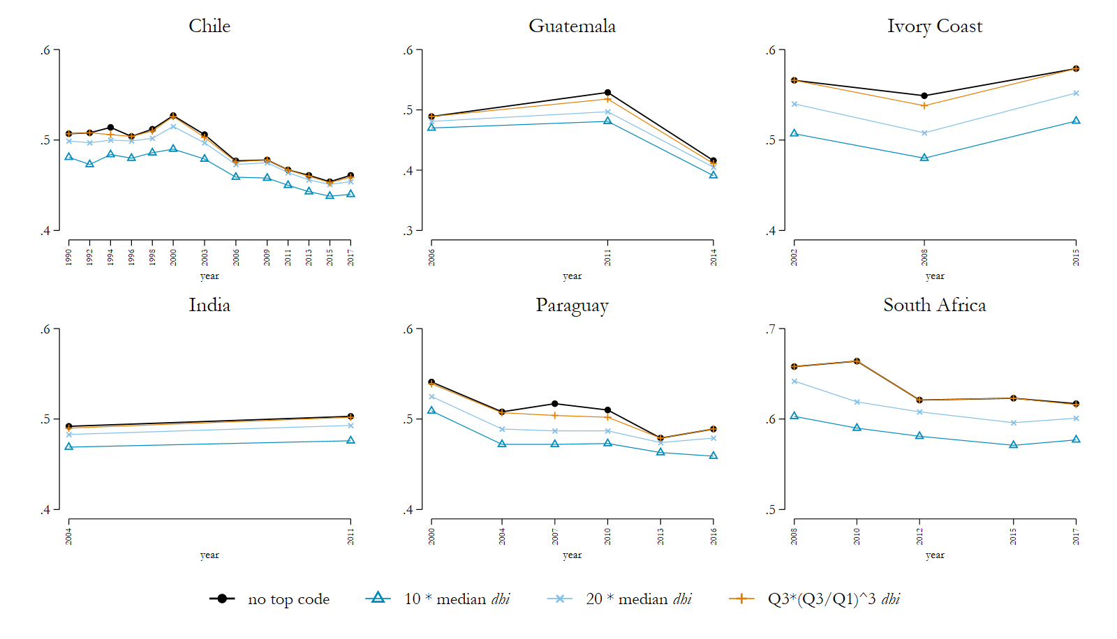
Note: See for all LIS datasets Figure 2 in the Appendix of LIS Technical Working Paper No. 9.
Source: Luxembourg Income Study (LIS) Database, accessed August 2020.

Figure 3: Alternative top coding procedures – Gini Index wage income (selected countries)

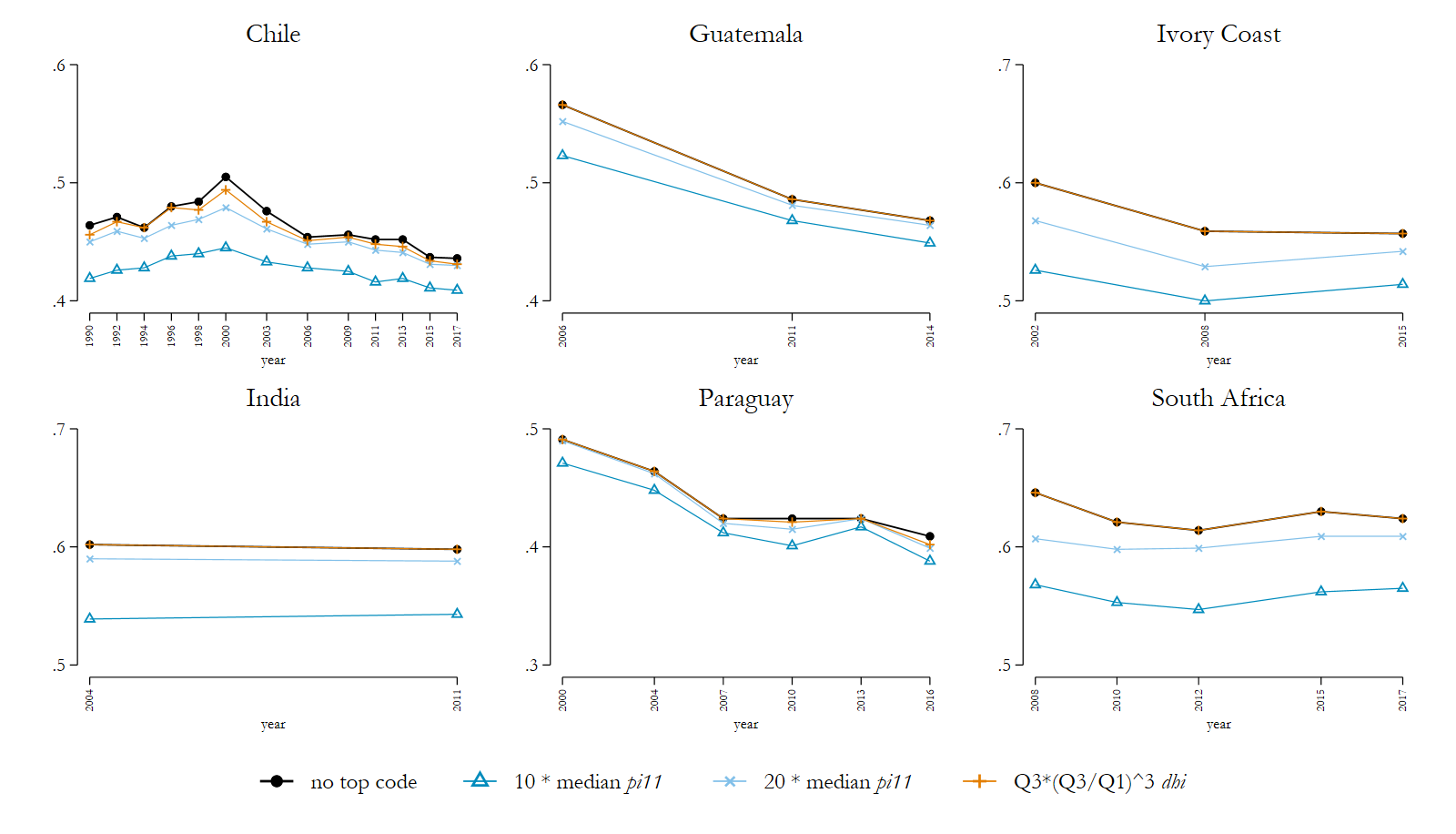
Note: See for all LIS datasets Figure 3 in the Appendix of LIS Technical Working Paper No. 9.
Source: Luxembourg Income Study (LIS) Database, accessed August 2020.

A second set of analyses concerns the bottom coding of values. The bottom coding of negative values has been a pragmatic decision in the past. As various data providers do not specifically collect losses in self-employment income or capital income, the LIS data was considered more comparable when negative values were set to non-negative values throughout the database. It is worth mentioning that this procedure is directly applied to disposable income and not at the level of the source income (more specifically, this means that when a loss in a household is offset by other income then no bottom coding is applied for this household). In order to keep the low values in the distributions for various income measures (and hence to distinguish them clearly from values 0), these values have previously been set to 1 % of the mean of equivalised disposable household income.

The previous method of setting negative values to 1 % of the mean is here contrasted with two measures: bottom coding at value 0 and bottom coding at the lower boundary for extreme values by the interquartile range, where the lower boundary is defined as Q1/(Q3/Q1)^3.

In a first step, we calculated the Gini Index for bottom coded distributions at value 0 and bottom coded values at the lower boundary of extreme values. These results are not shown here, as the Gini Index proved to be very insensitive to bottom coding procedures and in only a few cases changed by 0.1 % (e.g. 33.2 % instead of 33.3 %), and very rarely by 0.2 %.

Thus, in a second step, we tested the influence on a more critical measure towards low values, the Atkinson Index (Atkinson 1970), combined with a risk aversion parameter epsilon (ε) equal to 1.5. Note, however, that these three measures are not directly comparable as the computation of the Atkinson Index bottom coded at value 0 excludes negative and 0 values from the distribution. We perform this comparison at this stage to show that with a strict bottom code at value 0, very low reported values remain unmodified in the income distribution (after looking at the raw data these refer typically to very low capital incomes as the only income source collected). We therefore report the sensitivity of the Atkinson Index with epsilon (ε) equal to 1.5 with respect to these very low values and then contrast it to a more general approach, where we keep all observations in the sample but where we apply a positive lower bound on both negative and 0 values.

Figure 4 illustrates the sensitivity in the various bottom coding techniques for selected countries. First of all, due to the actual existence of very low values in the raw data, the calculations of the Atkinson Index became quite sensitive in some datasets, as can be seen, for example, in the extreme jumps in Italy and Norway. The alternative bottom coding techniques, applying 1 % of the mean or the lower boundary for extreme values, yield more stable patterns. Bottom coding at the boundary for extreme values strongly reduces the jumpy pattern of the Atkinson calculation, as compared to the 1 % of the mean. An additional line for the Gini Index allows for a direct comparison of the country-specific trends.

Figure 4: Alternative bottom coding procedures – Atkinson Index (ε=1.5) disposable household income (selected countries)

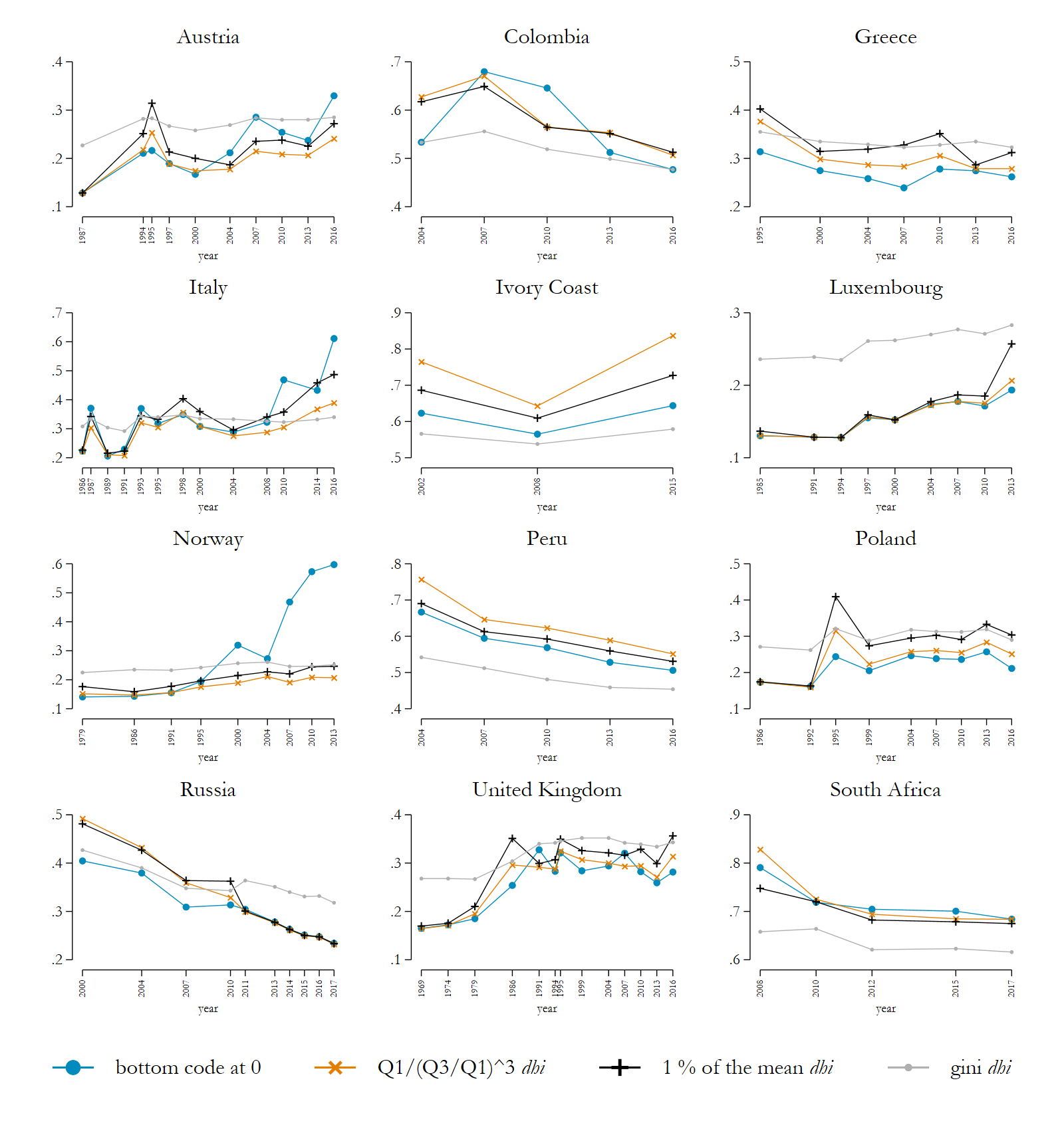
Note: See for all LIS datasets Figure 4 in the Appendix of LIS Technical Working Paper No. 9.
Source: Luxembourg Income Study (LIS) Database, accessed August 2020.

Particularly in emerging economies (see Ivory Coast, Peru, and South Africa) that have very unequal income distributions, the threshold for extreme values at the bottom is even lower than the threshold of 1 % of mean equivalised income. Hence fewer cases are treated in the extreme values approach and more inequality is kept in the data. The lower boundary for extreme values refers in 50 % of the datasets to a range between 2.8 to 5.8 % of mean equivalised dhi; 90 % are in a range between 1.3 to 8.5 % of mean equivalised dhi.

For further reference, we recommend to consult Neugschwender (2020), LIS Technical Working Paper No. 9, including a Table appendix with detailed dataset-specific statistics when applying different top and bottom coding procedures. Relatively large percentage shares at the bottom are in many cases due to 0 values in the raw data, which are also raised to the bottom coded value. This affects the 1 % of the median and the extreme values approach equally. After disregarding 0 values, only 15 datasets out of the 407 datasets in the LIS Database show percentage shares larger than 1 % when treated with the extreme values approach; 10 of these datasets show more than 1 % sample cases when treated with the 1 % of the mean bottom coding. At the top, treatment to top coding at the extreme values exceeds 0.1 % of sample cases in only 7 datasets, whereas the 10 times the median approach exceeds 1 % of the sample in 20 datasets.

Conclusion

After looking in depth at these figures we reinstated the necessity for applying top and bottom coding procedures for the LIS Key Figures and DART.⁴ This decision is motivated mostly in the context of cross-national comparisons, where we aim to preserve a ranked order of inequality between countries. Among the tested approaches we concluded that it is best to adopt the interquartile range as the new technique to first detect extreme values and then to apply the lower and upper boundary as a bottom and top code. The new measure affects inequality measures much less, as compared to the previous approach, but still smoothens inequality trends within and between countries by consistently reducing the influence of extreme values in the income distributions for inequality measures.

In line with LIS’ tradition of keeping the micro data as ‘original’ as possible we decided against implementing a technique to correct for these values in the micro data at this stage. At the same time, LIS cannot ask its data providers to systematically check these values. We therefore take a consistent approach to set these values to the lower and upper limit of the boundary. We emphasise at the same time that LIS keeps the reported values in the microdata and, as has always been its custom, leaves it up to the users to treat extreme values in the data.

LIS encourages its users to apply alternative procedures to better treat measurement error in the tails of the distributions with survey data. Such measures are, for example, re-weighting observations (e.g. Hlasny and Verme, 2018), semi-parametric approaches (e.g. Pareto distribution modelling for parametric tail (Cowell and Flachaire, 2007; Van Kerm, 2007)), or linking tax data to survey data as proposed by Blanchet et al. (2018).

¹ The author is grateful for various valuable comments and ideas received from Philippe Van Kerm, Piotr Paradowski, Teresa Munzi, and Daniele Checchi in completing this exercise of reassessing top and bottom coding practices at LIS. This article including an appendix can be downloaded as LIS Technical Working Paper No. 9.

² Another technique, trimming the upper end, was disregarded, as this technique would impact datasets where a top code has been applied. Thus by trimming the top end of the distribution we would further reduce inequality.

³ This formula is equal to, first, defining a new log transformed variable disposable household income, second, calculating the log values for the interquartile range, and finally using the exponential of the log values in the original income distribution before log transformation, EXP [log Q1 – 3*(logQ3 –logQ1)] for the lower boundary and EXP [log Q3 + 3*(logQ3 –logQ1)] for the upper boundary.

⁴ At this stage the method is limited to income measures. A similar practice cannot be applied for net worth as this latter contains a large share of negative values which affects the calculation of a robust interquartile range.

References

Atkinson, A.B. (1970), On the measurement of inequality, Journal of Economic Theory, Vol. 2, No. 3, pp. 244-263 ,https://doi.org/10.1016/0022-0531(70)90039-6

Atkinson, A. B., Lee Rainwater, L. and Smeeding, T. M. (1994), Income Distribution in European Countries, LIS working papers series, No. 121, available at http://www.lisdatacenter.org/wps/liswps/121.pdf, accessed: 3/2/2020.

Blanchet, T.; Flores I.; Morgan M. (2018), “The Weight of the Rich: Improving Surveys Using Tax Data”, WID.world Working Paper 2018/12, available at https://wid.world/document/the-weight-of-the-rich-improving-surveys-using-tax-data-wid-world-working-paper-2018-12/, accessed: 4/2/2020.

Cowell, F. A. and Flachaire, E. (2007), Income distribution and inequality measurement: The problem of extreme values, Journal of Econometrics, Volume 141, Issue 2, December 2007, pp. 1044-1072. https://doi.org/10.1016/j.jeconom.2007.01.001.

European Commission – Eurostat (2018), Working Group Labour Market Statistics, TF2: Income from main job (variable INCGROSS): Imputation bands, outlier detection, and dissemination plan, Luxembourg, June 13-14, available at https://circabc.europa.eu/webdav/CircaBC/ESTAT/labmarstatwg/Library/statistics_working/2018/1.%2013-14June%20(Section%20A_%20LFS)/2.%20Documents/Doc%2009%20Item%202.8%20Income%20from%20main%20job_INCGROSS.pdf, accessed: 2/2/2020.

Fritzell, J. (1992), Income Inequality Trends in the 1980’s: A Five Country Comparison?, LIS working papers series, No. 73, available at http://www.lisdatacenter.org/wps/liswps/73.pdf, accessed: 3/2/2020.

Gottschalk, P. and Smeeding, T. M. (1996), The International Evidence on Income Distribution in Modern Economies: Where Do We Stand? LIS working papers series, No. 137, available at http://www.lisdatacenter.org/wps/liswps/137.pdf, accessed: 3/2/2020.

Gottschalk, P. and Smeeding, T. M. (1997), Cross National Comparisons of Levels and Trends in Inequality, LIS working papers series, No. 126, available at http://www.lisdatacenter.org/wps/liswps/126.pdf, accessed: 3/2/2020.

Gottschalk, P. and Smeeding, T. M. (2000), Empirical evidence on income inequality in industrialised countries, in Atkinson, A.B. and Bourguignon, F. (eds.),Handbook of Income Distribution, vol. 1, Elsevier, pp. 261-307.

Hlasny, V.; Verme, P. (2018), Top Incomes and Inequality Measurement: A Comparative Analysis of Correction Methods Using the EU SILC Data, Econometrics, 6, 30.

Luxembourg Income Study (LIS) Database, http://www.lisdatacenter.org (multiple countries; July 15, 2020). Luxembourg: LIS.

Michael O’Higgins, M.; Schmaus, G. and Stephenson, G. (1985), Income Distribution and Redistribution, LIS working papers series, No. 3, available at http://www.lisdatacenter.org/wps/liswps/3.pdf, accessed: 3/2/2020.

Smeeding, T. M. (1997), American Income Inequality in a Cross-National Perspective: Why Are We So Different?, LIS working papers series, No. 157, available at http://www.lisdatacenter.org/wps/liswps/157.pdf, accessed: 3/2/2020.

Van Kerm, P., (2007), “Extreme incomes and the estimation of poverty and inequality indicators from EU-SILC,” IRISS Working Paper Series 2007-01, IRISS at CEPS/INSTEAD, available at: https://ideas.repec.org/p/irs/iriswp/2007-01.html, accessed: 4/2/2020.

Székely, M. and Hilgert, M. (1999), What’s Behind the Inequality We Measure? An Investigation Using Latin American Data, LIS working papers series, No. 234, available at http://www.lisdatacenter.org/wps/liswps/234.pdf, accessed: 3/2/2020.

Smeeding, T. M.; Schmaus, G. and Allegrezza, S. (1985), An Introduction to LIS – The Luxembourg Income Study, LIS working papers series, No. 1, available at http://www.lisdatacenter.org/wps/liswps/1.pdf, accessed: 3/2/2020.