Issue, No.11 (September 2019)

Using capital income to proxy family background: an application to measuring Inequality Of Opportunity

by Hugo del Valle-Inclán (University of Vigo)

This article draws from ECOBAS Working Paper No. 2019-01, “Estimating Inequality of Opportunity in Many New Periods: The Capital Income Approach” (June 2019), where the reader can find the detailed results.

What is inequality of opportunity and why does it matter?

When asked about the ideal distribution of income or wealth, people do not think of perfect equality. Instead, individuals seem to care about economic fairness, even if in actuality this may imply some inequality. A number of political philosophers and economists, from John Rawls to John Roemer, have tried to define what makes a distribution fair. In a nutshell, they propose that what should be equalized are not outcomes – whether income, wealth, educational attainment and such like – but the opportunities for attaining them. If when enjoying the same opportunities (think of them as choice sets) as anybody else, some individuals manage to attain greater levels of a certain outcome by means of personal effort, then no moral objection to such inequality could be put forward. Hence, in the field of inequality of opportunity, IOP henceforth, inequalities with respect to any outcome are deemed “fair” or “unfair” depending on where they stem from. Simply put, are considered fair those inequalities produced by factors individuals can choose – such as the degree of effort exerted – while unfair inequalities, on the contrary, arise from personal characteristics individuals cannot control – such as gender, race or family background. These personal characteristics, called circumstances, may indeed play a role in people’s social and economic development prospects, and this influence is judged ethically offensive on the grounds that these circumstances fall outside an individual’s responsibility. Of course, deciding which ones are the relevant circumstances is a normative task, as well as an essential step in the measurement of IOP.

The most common approach to empirically measuring IOP is to define a set of circumstances and to observe their joint distributions across a given outcome, most commonly income. With a representative sample, under the assumption of equality of opportunity (outcome distributed independently of circumstances), we should see no systematic inequality in outcomes between people of different circumstances. Nonetheless, in the real world we do observe a distance between this counterfactual ideal and the actual joint distributions, and that distance is what we call IOP. A more detailed overview of the underlying philosophy and measurement of IOP is presented in the article by Francisco H.G. Ferreira in this newsletter. Also in this publication, Maurizio Bussolo, Daniele Checchi and Vito Peragine have described an approach to estimating its long term evolution, while Paul Hufe and Andreas Peichl discuss a broader conception of what economic fairness entails.

Why would we want to use capital income to proxy family background?

The measurement of fair and unfair inequality has been attracting increasing attention in recent years. However, its empirical application is limited by the scarce availability of a key piece of information routinely included in the set of circumstances: the family background of individuals. For instance, in the LIS database we have information on parental education or occupation (variables typically employed to proxy family background) in only about 18 per cent of all waves.¹ In the case of the EU-SILC, another well-known database for the study of poverty and inequality, we have this kind of information for around 14 per cent of the waves.

This text explores how to overcome this data limitation. Instead of relying on the scarce availability of information on parental education or occupation we propose to use data on household capital income because this also proxies family background and it is widely available. In the case of LIS, we have information on household capital income for around 99 per cent of waves, while the EU-SILC approximates 93 per cent of them. Though the article on which this text is based employs only the EU-SILC database at this moment similar exercises have been carried out employing LIS data obtaining equivalent results. Naturally, nothing impedes applying this approach using any other database suitable for the study of poverty and inequality.

Why could capital income make a good proxy of family background?

In his famous book “Capital in the Twenty-First Century”, Thomas Piketty (2014) wrote about the return of what he dubbed patrimonial capitalism, referring to the importance of bequests in the determination of wealth. If patrimonial capitalism is truly back, then capital income could serve as a proxy for family background. And in addition to that, other mechanisms may be at play too: on the one hand, from the intergenerational mobility literature we know that more educated parents tend to transmit more social advantages, such as education, to their children (see for example Chetty et al., 2014, or Jäntti and Jenkins, 2015), while returns on investments appear to be linked to education and financial literacy, something we know from the portfolio literature (Von Gaudecker, 2015; Bucher-Koenen and Ziegelmeyer, 2011); on the other hand, savings and wealth ownership have been found to be largely determined by the intergenerational transmission of human capital, something explored by the wealth inequality literature (Charles & Hurst, 2003; De Nardi & Fella, 2017; Hällsten & Pfeffer, 2017; Hansen, 2014).

But wait, can we include a non-exogenous variable in the set of circumstances?

In Roemer’s definition (1998), only exogenous variables (exogenous meaning being beyond the influence of individual choice) may qualify as circumstances. Our proposal of including capital income in the circumstances’ set violates this principle. We defend our strategy on three grounds: a) capital income should be understood not as an income variable, but as a variable correlated to family background – to the extent that it accurately proxies parental features, the concern of it being within individuals’ control is lessened; b) to tackle this concern further we follow a procedure for “isolating” the exogenous component of capital income and to only then use it for the estimation of IOP; finally c), we perform an accuracy test of the IOP estimates produced, with satisfactory results. In sum, this method appears to constitute an informative approximation of IOP estimates obtained with a “standard” set of circumstances (i.e., including parental education), but it is much less limited by data availability. Using a measure of capital income to proxy family background is not likely to be preferable over employing data on parental characteristics; however, we suggest it is a useful alternative when the latter information is not available.

The capital income approach

Our project consists of three parts:

• We first construct an “exogenous” measure of capital income to be included in our set of circumstances that we will use to estimate IOP;
• Second, we test the accuracy of our approach by comparing IOP estimates obtained with a “standard” set of circumstances (i.e., including parental education) and our set (excluding parental education but including a measure of capital income). For this purpose we consider datasets in which information on both parental background and capital income is available. In the EU-SILC database these correspond to the waves of 2004 and 2010 only. We conclude that our approach is accurate to the extent that it returns similar results to those of the “standard” method that we adopted as our baseline;
• Once the reliability of our strategy has been assessed, we benefit from it and estimate IOP in datasets that do not have information on parental background, that is, most waves.

The database we use, the EUropean Survey of Income and Living Conditions, is a well-known and researched database for the study of inequality, poverty, and social exclusion. It offers harmonized data on income and circumstances at the individual and household level for up to 31 European countries in its most recent waves.

We employ the mean log deviation as inequality measure and use both a parametric and a non-parametric method to obtain lower bound estimates of ex-ante IOP (although for the sake of brevity we will only show the results of the non-parametric method in this text). Our outcome of interest is annual gross wage and we restrict our sample to individuals aged 30 to 59 whose main activity status is “at work”.

We keep in our sample only countries that were already present in the 2004 wave, thus excluding Bulgaria, Croatia, Malta, Romania and Switzerland. We also exclude from our analysis economies where the distribution of capital income was so skewed that only a tiny proportion of households received any capital income at all, since it impedes the grouping of individuals according to it. These economies are Estonia, Hungary, Ireland, Latvia, Lithuania, Poland and Slovakia. In addition, we do not estimate IOP in waves prior to 2007 in France, Greece, Italy, Spain and Portugal, because our outcome variable, gross annual wage, is not available in those datasets. Nonetheless, despite all these limitations, we are able to obtain a remarkable number of new IOP estimates.

For our set of circumstances we consider binary gender (2 groups), immigrant status (2 groups), and either parental education, for our baseline set of circumstances, or capital income, for the set of circumstances we propose (3 groups). Although a vector of three circumstances is without doubt smaller than the “true” vector, we make this choice in order to perform a stricter accuracy test of our method. Generally, the more circumstances are included in the set, the smaller the relative role of each one will be. For our case, this means that the difference of including parental education or capital income would be reduced as we increase the number of circumstances. Therefore, we believe that this reduced set is adequate for the task at hand, which is accuracy assessment. If our method performs satisfactorily with such a sparse number of circumstances, it is likely to perform better as the dimension of the set increases.

• Construction of an “exogenous” measure of capital income

We can think of wealth ownership and capital income as determined by two elements: a dynastic component, the product of advantages acquired through birth such as access to good education and bequests, and a meritocratic one, coming resulting from effort exerted during our lifetime. To reduce the influence of the latter component we will follow a procedure endeavouring to isolate the former, and only then include it as a measure of capital income in our set of circumstances’ set. This procedure consists of running an OLS regression of per capita gross capital income of households against a number of individual characteristics representing individual effort (namely education and occupation), and position in the life cycle (age). A time dummy is included as well.² Then, after obtaining the residuals ϵ_i from (1), which can be seen as the value of per capita capital income once the influence of non-dynastic factors has been removed, we construct a discrete variable grouping individuals according to the size of these residuals.

pckinc_i = β₀ + β₁ education_i + β₂ occupation_i + β₃ age_i + β₄ year + ϵ_i       (1)

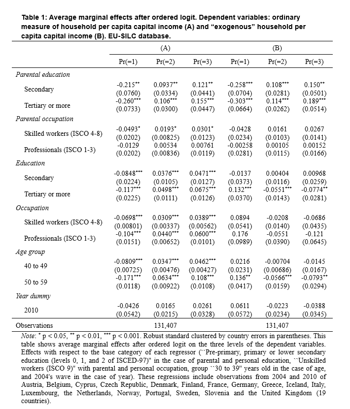
Now that we have constructed an “exogenous” measure of capital income, let us look at how it is related to parental features. Table 1 shows the average marginal effects obtained after two ordered logistic regressions. In the first regression, column (A), the dependent variable is an ordinary measure of capital income (including both the dynastic and meritocratic components), and the second one, column (B), shows our “exogenous”, or dynastic, measure. These regressions are run using pooled cross-sectional data of our subset of 19 countries, including observations from both the 2004 and 2010 waves. In short, we can see that capital income appears to be related to parental education and that this relationship becomes stronger if we consider our “exogenous” measure. Also, by following our isolation procedure, it seems that we have managed to reduce the influence of non-dynastic variables, as seen by comparing the results in (A) and (B). Therefore, we conclude that our proxy of family background might be a valid alternative to parental information and can proceed to use it to estimate IOP.

• Testing the accuracy of the approach

Using the EU-SILC database we obtain the estimates of absolute IOP shown in Figure 1, referring to 2004 and 2010. On the vertical axes are estimates obtained using the “baseline” set of circumstances; on the horizontal axes are shown the “capital” estimates. The closer these points are to the diagonal grey line, the more similar both kinds of estimates are. They are generally similar, and we find pairwise correlations close to 1.

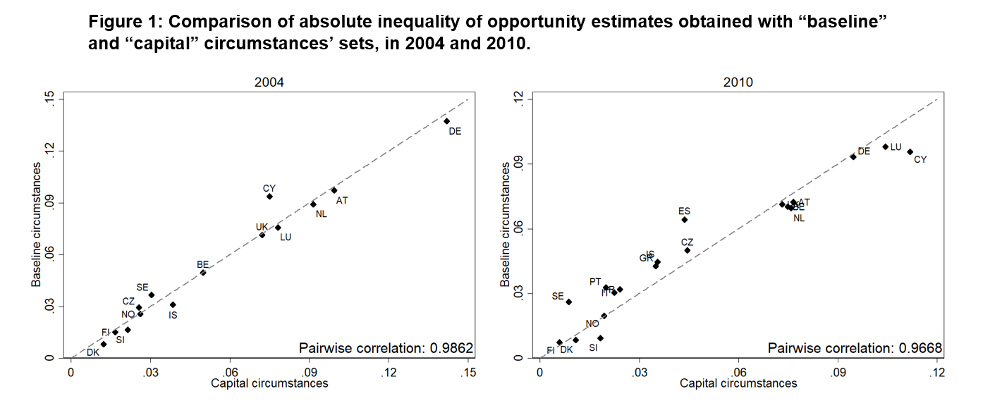
Source: EU-SILC.

A common use of cross-country IOP measures are international rankings. Figure 2 shows comparisons of IOP ranks. It would be an interesting feature of the capital income approach to be a rank-preserving method with respect to baseline estimates, although it is not the case. Nevertheless, the rank correlations between our “baseline” and “capital” estimates are also close to 1, meaning that if a country ranks high (low) according to the “baseline” IOP measure, it will rank high (low) as well if measured with the capital income approach, and vice versa. For a more comprehensive accuracy test and a robustness analysis, the reader is referred to the working paper version of this article.

Source: EU-SILC.

• Benefiting from the approach

Once we have tested the reliability of the capital income approach we can proceed to take advantage of it and obtain IOP estimates for almost the full extent of the EU-SILC database. Figure 3 shows, to the best of our knowledge, the largest number of IOP estimates of European countries produced so far. These IOP estimates have been obtained using a non-parametric approach and consist of relative IOP measures. The advantage variable is gross annual wage and the inequality measure employed is the mean log deviation. Confidence intervals are shown as grey areas, which have been calculated with standard errors computed via bootstrapping (400 replications) stratified by country, year and region. This figure includes as well IOP estimates obtained with our “baseline” circumstances, in which confidence intervals are displayed as red bars, for the only periods for which these are available, namely 2004 and 2010. This allows to rapidly assess the similarity between the “baseline” and “capital” estimates and illustrates how large is the number of new data points obtained thanks to the capital income approach.

Figure 3: Evolution of relative IOP in Europe, estimated with the “capital” set of circumstances

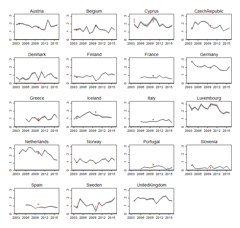
Notes: Confidence intervals shown as grey areas, which have been calculated with standard errors computed via bootstrapping stratified by country, year and region (400 replications). Confidence intervals of IOP estimates obtained with “baseline” circumstances displayed in red bars. The advantage variable is gross annual wage, the inequality measure employed is the mean log deviation, and the estimation approach is non-parametric.
Source: EU-SILC.

Summing up

This article has introduced a strategy to estimate IOP that does not rely on the availability of data on parental characteristics. After testing the accuracy of our method we conclude that it is sufficiently reliable to be used in cases where we lack information on parental background, thus enabling us to obtain many new IOP estimates. Possible uses of the increased number of data points available include, for instance, studying the relationship of IOP with institutions, economic growth or electoral outcomes. It also helps to obtain historical estimates, allowing to use old datasets that do not contain parental data.

¹ As of the time of writing this article.

² Previous versions also included as regressors dummies of population density, to account for the differences between rural and urban wealth, and mating, for the effect of marriages. Since the results do not change, they have been removed for the sake of simplicity.

References

Bucher-Koenen, T., & Ziegelmeyer, M. (2011). Who Lost the Most? Financial Literacy, Cognitive Abilities, and the Financial Crisis. European Central Bank Working Paper Series 1299.

Charles, K. K., & Hurst, E. (2003). The Correlation of Wealth across Generations. Journal of Political Economy, 111(6), 1155–1182.

Chetty, R., Hendren, N., Kline, P., & Saez, E. (2014). Where is the Land of Opportunity? The Geography of Intergenerational Mobility in the United States. Quarterly Journal of Economics, 129(4), 1553–1623.

De Nardi, M., & Fella, G. (2017). Saving and wealth inequality. Review of Economic Dynamics, 26, 280–300.

Hällsten, M., & Pfeffer, F. T. (2017). Grand Advantage: Family Wealth and Grandchildren’s Educational Achievement in Sweden. American Sociological Review, 82(2), 328–360.

Hansen, M. N. (2014). Self-Made Wealth or Family Wealth? Changes in Intergenerational Wealth Mobility. Social Forces, 93(2), 457–481.

Jäntti, M., & Jenkins, S. P. (2015). Income Mobility. In A. B. Atkinson & F. Bourguignon (Eds.), Handbook of Income Distribution(Vol. 2, pp. 807–935). Amsterdam: Elsevier North Holland.

Piketty, T. (2014). Capital in the Twenty-First Century. Cambridge: Harvard University Press.

Roemer, J. E. (1998). Equality of Opportunity. Cambridge: Harvard University Press.

Von Gaudecker, H. M. (2015). How Does Household Portfolio Diversification Vary with Financial Literacy and Financial Advice? Journal of Finance, 70(2), 489–507.