Issue, No.27 (September 2023)
The ‘lissyrtools’ R package V0.1: Functions for computing inequality estimates in the LISSY environment
Using R in LISSY might not be the easiest way of obtaining inequality estimates. The code can sometimes feel verbose when compared to other software and users might need to use their own functions and code for rather basic operations. At the same time, analyzing income and wealth distributions requires substantive knowledge to be able to assess important methodological decisions (e.g. equivalence scales, adjusting by CPI and PPP, dealing with outliers). These two factors might create an entry barrier for many users who would like to use R and aren’t proficient in the software and/or the methods for analyzing income and wealth distributions.
The ’lissyrtools’ R package aims to make the use of R in LISSY simpler. It provides a set of commonly used functions that can easily reproduce LIS estimates such as those in DART, IKF and in the Compare.It dashboard.1 The package is currently in Beta (0.1) version. It is installed in LISSY and users can download it locally from the LIS GitHub repository.2 If you try it and want to give us your feedback, please send us an email to usersupport@lisdatacenter.org.
The package contains basic types of functions:
- ‘read_’ functions to read the data;
- ‘transform_’ to clean variables;
- ‘print_’ to produce estimates;
- ‘plot_’ to produce plots.
The function definition and documentation can be found in the package website.
The chunks of code below reproduce the computation of the DART dashboard estimates for a subset of files. The code can be copy-pasted from this GitHub Gist into the LISSY interface.
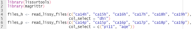
Like all R packages, we can load it with ‘library()’. The script below also loads ‘magrittr()’, which is used to pipe functions. ‘read_lissy_files()’ is then used to read the data.3 All the files passed as an argument need to be at the same level (i.e. either household or person-level). This level is stored in the returned object (‘files_h’ and ‘files_p’ below) and then used by other functions.4 In this example code, we read multiple files from the Canadian series.
The ‘col_select’ parameter can be used to subset the variables read. ‘read_lissy_files()’ always reads key variables such as ‘hid’, ‘nhhmem’ and weights, even if they are not passed as an argument.
A commonly performed computation using LIS data is to merge the household and person level files. This allows users to have all the household variables matched to individuals. ‘lissyrtools’ makes this task easy with ‘merge_dataset_levels()’. This function checks that the names of the files in both the household and person-level objects (‘files_h’ and ‘files_p’ in the example) are the same and then proceeds to iterate over them to merge them.

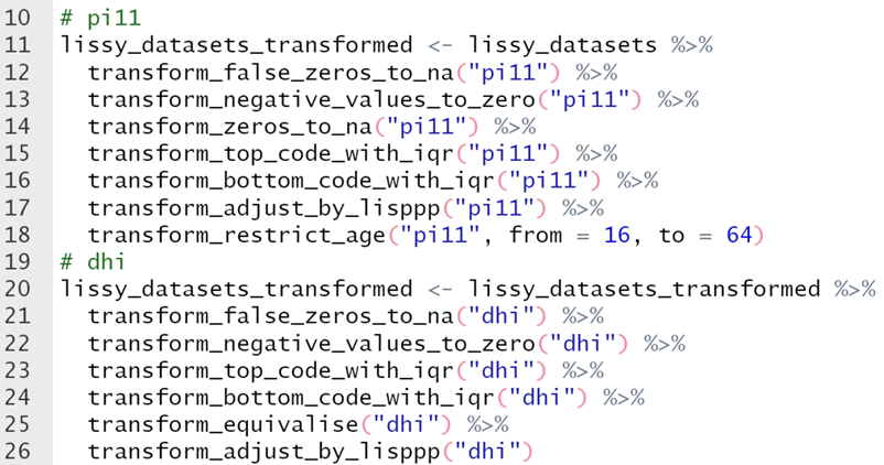
There are so far eleven ‘transform_’ functions that should make the task of processing data easier. Eight of these are shown in the code below. For more detail about the functions use and definition, check the reference section of the package website.
In the code below, we are performing the same data processing we would do to compute the LIS Gini estimates published in the DART dashboard for ‘wage income’ (‘pi11’) and ‘disposable household income’ (‘dhi’). In the case of ‘wage income’, this consists of:
- Treating a variable of all 0s as all missing values;
- Recoding negative values and 0s to missing values, so they are not included in the computations;
- Applying a top and bottom coding using the Interquartile range;
- Adjusting the variable by CPI and PPP;
- Using only individuals with ages between 16 and 64 (both included).
For ‘wage income’ we keep the 0s, but we apply an equivalization using the square root of the number of household members.
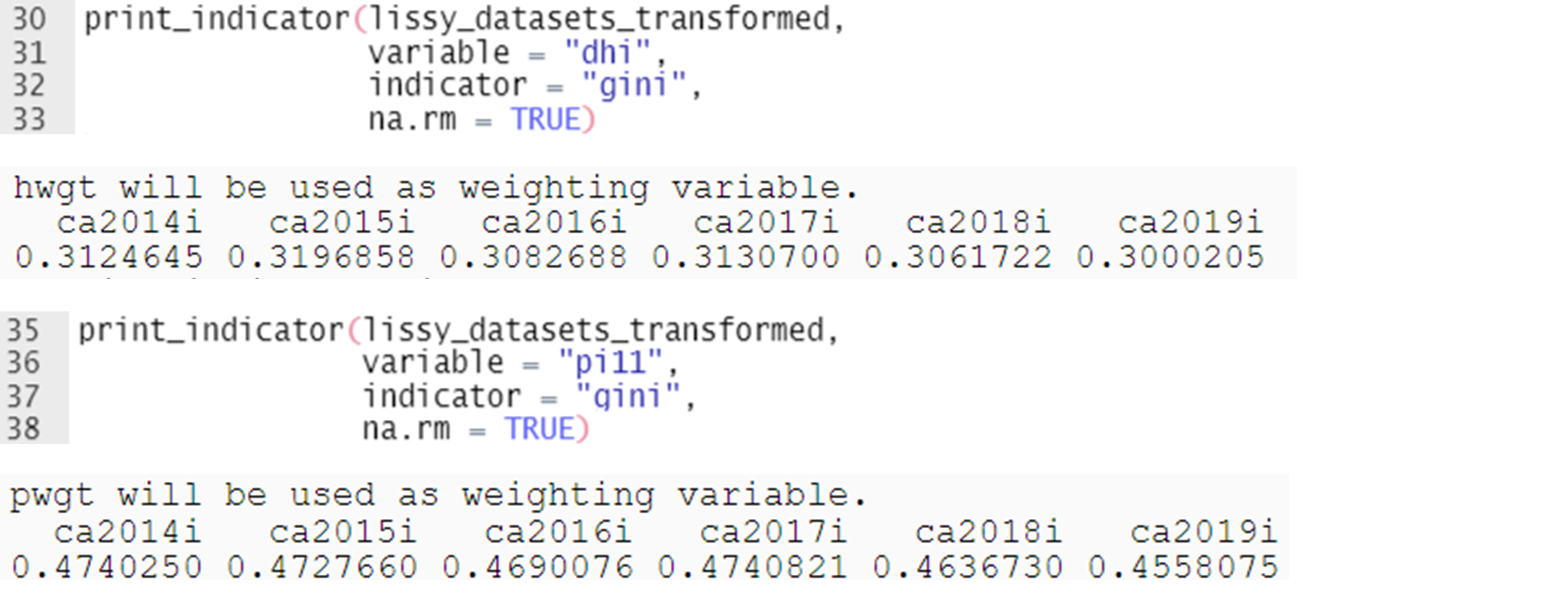
The next step is to produce estimates. This can be done with the ‘print_’ functions. The call to ‘print_indicator()’ below computes the Gini Coefficient (indicator = “gini”) for the ‘dhi’ and ‘pi11’ variables, which we read and cleaned above. The function currently supports the following indicators: ‘mean’, ‘median’, ‘ratio’, ‘atkinson’ and ‘gini’. You can find more details in the function reference.
When we print the ‘gini’ of ‘dhi’, a message informs us that ‘hwgt’, the household-level weight, was used to weight the variable. This is because ‘lissyrtools’ recognizes ‘dhi’ as a household-level variable. If the variable name is not that of a standard variable, the function would have required an additional argument (‘variable_level’). Similarly, when computing an indicator for ‘pi11’, the function uses ‘pwgt’ instead of ‘hwgt’ as a weighting variable. The results of ‘print_indicator()’ are returned as a named vector, which can then be used for subsequent operations.
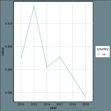
Last, we can use ‘plot_indicator()’ to compute and plot indicators. This function calls ‘print_indicator()’ behind the lines and takes the additional step of plotting the results. ‘plot_indicator()’ takes the same arguments as ‘print_indicator()’ and also has a ‘plot_theme’ parameter for passing ‘ggplot2’ themes. The default theme (as displayed below) uses the LIS colors.

1 In fact, the LIS processes to compute those estimates use functions from ‘lissyrtools’.
2 This can be useful if users want to try the package functions on the LIS sample files.
3 ‘read_lissy_files()’ works only in LISSY. To read data locally you should use ‘read_lissy_files_locally()’
4 For example, the ‘print_’ family of functions use the level of the data.frame and the specified variable to pick a default weight variable.