Issue, No.13 (March 2020)
Estimates of Wealth Inequality and Right Tail Coverage: An Illustration of Oversampling in the Survey of Consumer Finances
This article is an abridgement of Kennickell, A. (2019). ‘The tail that wags: differences in effective right tail coverage and estimates of wealth inequality’. The Journal of Economic Inequality , vol. 17, pp. 443-459, https://doi.org/10.1007/s10888-019-09424-8.
Introduction
In household surveys, it is rare that every sample member is willing to participate. A given segment of an observed distribution may be over- or under-represented in a survey relative to the population, either because of random variation in the sampling process or because of differences across the spectrum of survey sample members in their willingness to participate in the survey. If differences in willingness of sample members to participate are not statistically independent with respect to the analytical dimension(s) of interest, then the measured distribution will differ from what would be estimated from the full sample and many classes of estimates made on such data would be biased.
This article focuses on the sensitivity of survey-based estimates of wealth inequality to the quality of the measurement of the upper tail of the distribution. Such distortions in the measurement of the upper tail of many economic distributions may be especially problematic, because this tail is often highly skewed, as in the case of income or wealth—and in the absence of external bounding information, the distribution is open-ended. In the case of wealth, even within the group of individuals captured in the Forbes list of the 400 wealthiest individuals in the U.S., there is very substantial variation; for example, the minimum wealth to qualify for membership in the list in 2013 was $1.3 billion while the maximum holding among the group was $72 billion.1 Relative to the $81,200 median U.S. household wealth in 2013, $72 billion is extraordinarily remote. Indeed, the total wealth of the wealthiest few members of the Forbes list possessed more net worth than the least wealthy half of all U.S. households together, as measured in the Survey of Consumer Finances (SCF).
The article presents two of the illustrative examples in Kennickell (2019) to highlight some of the problems in making comparisons of wealth inequality measures when there are specific defects in the measurement of the upper tail of the distribution. For motivation, the article first presents an example based on two sets of time series estimates of wealth shares from the 2013 SCF: one computed from the full SCF sample, including a component that oversamples wealthy households, and the other computed without that additional sample. Next, the 2013 SCF is used to simulate an assortment of distortions in the upper tail of the wealth distribution that might be present in a survey. A final section concludes and outlines a potential research program for improving comparability of wealth measurement across surveys and within waves of a given survey.
Illustrative Example: Survey of Consumer Finances
The SCF is particularly helpful for illustrating the effects of differences in the effective coverage of the upper tail of the household wealth distribution on estimates of wealth concentration. The SCF is based on a dual-frame sample design, including both an area-probability sample (APS) and a list sample (LS).2 Households in the APS are selected with equal probability and stratified to yield a sample with a balanced geographic distribution. The LS is designed specifically to strongly oversample wealthy households. In the final sample, the APS and the LS are combined for analysis through the construction of weights that maximize the strengths of each sample.
The APS provides robust national representation of broadly-distributed characteristics. But an equal-probability sample contains, on average, only 1% of its observations among the wealthiest 1%. For example, an APS of 7,900 sample elements (as in the 2013 SCF) would, on average and assuming all cases are in scope and agree to participate, include only 79 elements to represent the wealthiest 1%. The use of random sampling also implies that the number of such wealthy cases selected would vary; for example, there is a 95% probability that the number of cases in this group would differ from the average figure by no more than about 14.
Hence, the LS is specifically intended to supplement the small expected number of wealthy respondents obtained in the APS, to identify wealth-related nonresponse and to support meaningful adjustments for such differential nonresponse.3 The sample is based on statistical records derived from individual income tax returns by the Statistics of Income Division of the U.S. Internal Revenue Service. A combination of models is used to project capital income and other characteristics observed in those records to an approximation of wealth, a “wealth index”, which is used to stratify the sample.
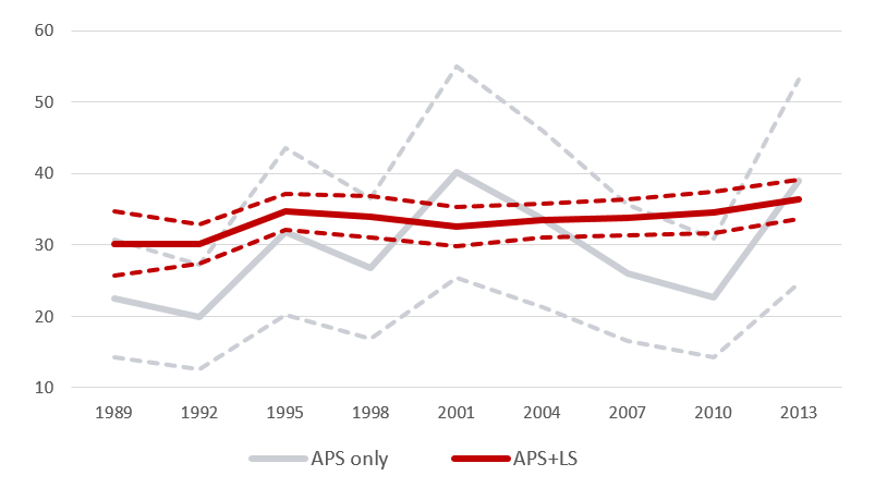
Because the LS is based ultimately on information from personal income tax returns, the unit of observation—the “tax unit”—does not necessarily align with the household concepts of the APS. In practice, there appears to be only a very small difference at the top of the income or wealth distribution, but differences are substantially greater differences at lower levels. The LS can include only people who filed individual tax returns, and many low-income households do not file returns. In addition, experience indicates that households with relatively lower income or wealth are more likely to have important secondary filers, especially spouses who file their tax returns separately. Thus, the LS focuses very heavily on the top 1% of the distribution of the wealth index and includes only a relatively small measure of other cases to facilitate the integration of the two samples. To highlight the importance of the LS in inequality measurement, Figure 1 shows the estimated wealth share (and its 95 percent confidence interval) of the wealthiest 1% for the surveys conducted between 1989 and 2013, using the combined APS and LS samples, and the same estimates made using only the APS.
Fig. 1: Wealth share of the wealthiest 1% and associated confidence intervals; combined APS and LS and APS alone; SCF, 1989–2013
Alternative Measures Using Simulated Populations
In Kennickell (2019), we test five experimental samples in order to test the extent of effective coverage of the upper tail of the wealth distribution. These variations span a plausible range of problems in measuring the upper wealth tail in the case of most surveys without strong controls over that population through the sample design or weighting adjustments. The simulations operate by altering the weights for some observations in the 2013 SCF combined sample to impose patterns of “non-observation” on the upper tail of the distribution of household wealth. Table 1 summarizes the five experimental scenarios. For further technical information and illustration see Kennickell (2019).
Table 1: Specification of experimental samples
| Item | Experiment 1 | Experiment 2 | Experiment 3 | Experiment 4 | Experiment 5 |
|---|---|---|---|---|---|
| Population addressed | Wealthiest 1% | Wealthiest 1% | Wealthiest 1% | Wealthiest 1% | Wealthiest 5% |
| Average weight reduction | 50% | 50% | 90% | 100% | 90% |
| Pattern of decay | Flat | Linear | Exponential | Flat | Exponential |
By design, none of the experimental samples involves oversampling in the upper tail of the wealth distribution, unlike the combined SCF sample. To give an indication of how much difference the oversampling alone makes in the precision of the estimated inequality measures considered, a set of random replicates for the full combined sample was constructed ignoring the structure imposed by the oversampling. Thus by construction, estimates in this case differ in expectation from the combined sample estimates only in the width of the confidence intervals.
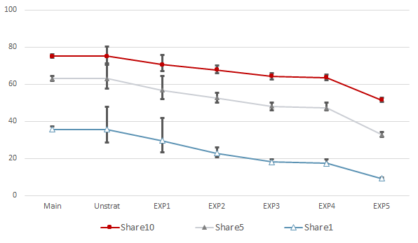
For each of the samples, Fig. 2 shows estimates of the wealth share for the wealthiest ten, five and 1%, along with the associated confidence intervals. Although the estimates of the share of the wealthiest 10% from the experimental samples show the smallest absolute and proportional bias among the share measures shown, the difference between the value estimated using the combined APS and LS samples and the estimated value for the fourth experiment is about 12 percentage points. As one might expect in light of the results presented earlier in this paper, the range of estimates for the wealthiest 1% is much wider: the estimated value for the fourth experiment is less than half the estimated value for the combined sample. The estimated confidence intervals for the all the experiments except the first give a misleading impression of the reliability of the share estimates. Thus, these results suggest that comparisons of such straightforward estimates of wealth shares for the upper tail across time or across surveys are unlikely to be informative, except where there is minimal nonresponse and a sufficiently large sample, or where there is a strong control on the measurement of that tail.
Fig. 2: Share of total wealth held by the wealthiest 10%, 5%, and 1%; combined APS and LS, unstratified combined sample and experiments 1–5; SCF, 2013
Conclusions and a Way Forward
Kennickell (2019) explored the sensitivity of a variety of indicators of the distribution of wealth. Results for one of those indicators considered here—wealth shares of various percentile groups—strongly indicate that in the absence of effective controls on the measurement of the upper tail of the wealth distribution, great caution should be the rule in the interpretation of commonly used measures of wealth distribution from a given survey, comparison of such measures across the waves of the survey, and perhaps even more strongly, comparison across independently designed and managed surveys. Among the inequality measures considered in Kennickell (2019), only the ratio the 95th to the 25th percentile of wealth and the ratio of the 90th to the 25th percentile of wealth appear to be reasonably reliably informative when estimated from surveys with biases in the measurement of the top of the distribution.
Without access to reliable data with information on characteristics closely related to wealth, such as income tax data, it is very difficult at best to develop a sample that provides sufficiently effective coverage of the upper tail of the wealth distribution to yield purely survey-based and reasonably stable estimates of wealth concentration. Although the SCF appears to do very well in addressing the relevant measurement concerns, even it shows some signs of deviation at the highest levels of the wealth distribution, and the sampling error in estimates disproportionately influenced by that tail, though not enormous, is also not negligible (see Kennickell, 2017). There is room for improvement in all wealth surveys.
Improvement can be made by using administrative data for sampling or for weighting adjustment, as in the SCF, the Encuesta Financiera de las Familias and the Enquête Patrimoine, or in the case of countries with reliable wealth register data, by replacing some or all of the survey measures. For example, Saez and Zucman (2016) take a related approach of estimating wealth entirely from administrative data on income and related measures. But these approaches are not possible for every survey of wealth. In other cases, some degree of modeling may be helpful in improving the measurement of the upper tail. Using only the observed data in the Austrian implementation of the Household Finance and Consumption Survey for 2010, Eckerstorfer et al. (2016) estimated a Pareto distribution for the upper tail of using information from a range of data from about the 70th to 99th percentiles of the observed data and they “recover” substantial additional wealth. When administrative data are not available for direct use, it may still be possible to obtain estimates of distributional curvature for wealth or a proxy from such data and apply those estimates to adjust the survey weights. Other external estimates, such as “rich lists” may also be used to adjust the weighting of observed data or to “impute” unobserved wealth. Vermeulen (2016, 2018) used Forbes and similar data on wealthy individuals in conjunction with survey data for several countries to estimate Pareto distributions to describe the augmented data. Bach et al. perform a similar exercise with a set of surveys that perform oversampling and find incorporating such external information make only a small difference in those cases. Even national accounting data on wealth may be useful in developing improved estimates, for example, by estimating Pareto distributions conditional on the total implied wealth equalling the aggregate value. In my view, finding the most robust approach that is applicable to many surveys should be the highest priority for research in this direction.
1See https://www.forbes.com/forbes-400/list/9/#version:static (accessed May 2019) for the most recent such information.
2See Kennickell (2017) for a detailed discussion of the SCF samples and for references to other technical research and information about the survey.
3The survey explicitly omits individuals who appear on the Forbes list of the 400 wealthiest people in the US.
References
| Bach, S., Thiemann, A., and Zucco, A. (2015), The Top Tail of the Wealth Distribution in Germany, France, Spain, and Greece. DIW Discussion Papers, No. 1502. |
| Eckerstorfer, P., Halak, J., Kapeller, J., Schütz, B., Springholz, F., Windauer, R. (2016), Correction for the missing rich: an approach to wealth survey data. Rev. Income Wealth. 62, 605–627. |
| Kennickell, A.B. (2019), The tail that wags: differences in effective right tail coverage and estimates of wealth inequality, Journal of Economic Inequality, 17: 443. https://doi.org/10.1007/s10888-019-09424-8 |
| Kennickell, A.B. (2017), Lining up: survey and administrative data estimates of wealth concentration. Statistical Journal of the International Association for Official Statistics, 33, 59–79. |
| Saez, E., Zucman, G. (2016), Wealth inequality in the United States since 1913: evidence from capitalized income tax data. Q. J. Econ. 131, 519–578. |
| Vermeulen, P. (2016), Estimating the top tail of the wealth distribution. Am. Econ. Rev. Pap. Proc. 106(5), 646–650. |
| Vermeulen, P. (2018), How fat is the top tail of the wealth distribution. Review of Income and Wealth. 64, 357–387. |